performance

library(lazymatrix)
#> 
#> Attaching package: 'lazymatrix'
#> The following object is masked from 'package:base':
#> 
#>     norm

Performance of `lazymatrix`

In this vignette, we discuss the main reason for lazy computation, namely the increase in performance. Assume X as the sparse data matrix containing fetures, lazy_X the LazyMatrix object and A is the normalized version obtained using base::scale(X). We use the package bench to microbenchmark the computation time of matrix-vector multiplication, hence comparing the operation lazy_X%*%b against A%*%b. Thereafter, we look at memory allocation, where we compare storing the LazyMatrix object and the normalized object.

Helper Functions

For these experiment, we need a set of helper functions. As the main use-case is working with sparse data, we define a helper forgenerating sparse matrices create_sparse_matrix_col() which allows for adjusting the parameter sparsity_col so the proportion of elements that are non-zero within each column. For simplicity, this parameter will be called $\alpha$ , Then, we use the helper bench_multiply() where we define the LazyMatrix object for the input matrix, normalize it and then we benchmark matrix-vector multiplication. The function benchmark_memory() is written in a similar way, though it uses utils::object.size() to measure memory allocation of an object, the lazy and the dense. Lastly, two helper functions which are used for using consistent themes for ggplot2 throughout the vignette.

library(Matrix)
library(bench)
library(dplyr)
#> 
#> Attaching package: 'dplyr'
#> The following objects are masked from 'package:stats':
#> 
#>     filter, lag
#> The following objects are masked from 'package:base':
#> 
#>     intersect, setdiff, setequal, union
library(ggplot2)
#--------------------------------------------------
# Sparse matrix generator
#--------------------------------------------------
create_sparsematrix_col <- function(n, p, sparsity_col) {
  # sparsity_col = fraction of non-zeros PER COLUMN
  # So each column has round(sparsity_col * n) non-zero entries
  n_nonzero_col <- round(sparsity_col * n)

  i_all <- c()
  j_all <- c()

  for (col in 1:p) {
    i_col <- sample(1:n, n_nonzero_col, replace = FALSE)
    i_all <- c(i_all, i_col)
    j_all <- c(j_all, rep(col, n_nonzero_col))
  }

  pairs <- unique(data.frame(i = i_all, j = j_all))
  x     <- rnorm(nrow(pairs))

  Matrix::sparseMatrix(
    i    = pairs$i,
    j    = pairs$j,
    x    = x,
    dims = c(n, p)
  )
}

#--------------------------------------------------
# Benchmark function Computation Time
#--------------------------------------------------
bench_multiply <- function(sparse_matrix, b) {
  A <- scale(sparse_matrix, center = TRUE, scale = TRUE)
  X <- LazyMatrix(sparse_matrix, "sd", "mean")
  bench::mark(
    dense_product = { A %*% b },
    lazy_product  = { X %*% b },
    check         = FALSE,
    min_iterations = 20
  )
}

#--------------------------------------------------
# Benchmark function for Memory Allocation
#--------------------------------------------------

benchmark_memory <- function(M) {
  dense_size <- tryCatch({
    A_dense <- scale(as.matrix(M), center = TRUE, scale = TRUE)
    mem     <- as.numeric(utils::object.size(A_dense)) / 1024^2
    rm(A_dense); gc()
    data.frame(method = "Dense", success = TRUE, mem_MB = mem)
  }, error = function(e) {
    message("Dense error: ", e$message)
    data.frame(method = "Dense", success = FALSE, mem_MB = NA)
  })

  lazy_size <- tryCatch({
    X_lazy <- LazyMatrix(M, "sd", "mean")
    mem    <- as.numeric(utils::object.size(X_lazy)) / 1024^2
    rm(X_lazy); gc()
    data.frame(method = "Lazy", success = TRUE, mem_MB = mem)
  }, error = function(e) {
    message("Lazy error: ", e$message)
    data.frame(method = "Lazy", success = FALSE, mem_MB = NA)
  })

  bind_rows(dense_size, lazy_size)
}

#--------------------------------------------------
# Plot Theme used throughout the thesis for ggplot2
#--------------------------------------------------
thesis_theme <- function(base_size = 12) {
  theme(
    panel.background = element_rect(fill = "white", colour = NA),
    plot.background  = element_rect(fill = "white", colour = NA),
    panel.grid.major = element_line(colour = "grey85"),
    panel.grid.minor = element_line(colour = "grey92"),
    panel.border     = element_rect(colour = "black", fill = NA, linewidth = 0.8),
    text             = element_text(size = base_size),
    axis.text        = element_text(size = rel(1.01)),
    axis.text.x      = element_text(size = rel(1.01), angle = 45, hjust = 1)
  )
}

#--------------------------------------------------
# Plot Theme used throughout vignettes for ggplot2
#--------------------------------------------------

vignette_theme <- function(base_size = 12) {
  theme_minimal(base_size = base_size) +
  theme(
    # Subtle background strip for facet labels
    strip.background  = element_rect(fill = "#f0f0f0", colour = NA),
    strip.text        = element_text(face = "bold", size = rel(0.95)),

    # Thin, unobtrusive grid
    panel.grid.major  = element_line(colour = "grey88", linewidth = 0.4),
    panel.grid.minor  = element_blank(),

    # Light border just around facet panels
    panel.border      = element_rect(colour = "grey70", fill = NA, linewidth = 0.5),
    panel.spacing     = unit(0.8, "lines"),

    # Legend inside or on top saves horizontal space in HTML
    legend.position   = "top",
    legend.key.width  = unit(1.8, "lines"),

    # Axis: no need to rotate if labels are short
    axis.text.x       = element_text(size = rel(0.9)),
    axis.text.y       = element_text(size = rel(0.9)),
    axis.title        = element_text(size = rel(0.95)),

    plot.margin       = margin(8, 12, 8, 8)
  )
}

Results of Computation Time Benchmark

We run the experiment as follows: let n be the number of rows of the sparse matrix which we let be constant for all matrices at n <- 10000. In statistics, the number of rows usually denotes the number of observations and the columns the features. Hence, letting n be constant and augmenting the columns p reflects the experiment of adding features to an existing dataset. Apart from dimensionality, the experiment also depends on sparsity, so the proportion of non-zero elements for every column. We test for three levels of sparsity, 5 %, 0.1 % and 0.01 %. A rule of thumb when working with sparse matrices, is that the larger the dimensionality, the lesser the sparsity usually.

Then, we run the benchmark function for matrix-vector multiplication defined above for every p and every sparsity. The results are therafter translated into seconds and we keep them in a tibble which is used to graph the result.

#--------------------------------------------------
# Parameters (smaller for testing)
#--------------------------------------------------
n              <- 10000
sparsity_cols  <- c(0.05, 0.001, 0.0001)
p_values       <- c(50, 100, 200, 500, 1000, 2000)

#--------------------------------------------------
# Run benchmarks
#--------------------------------------------------
results <- list()
counter <- 1

for (sc in sparsity_cols) {
  cat("Running sparsity_col =", sc, "\n")
  for (p in p_values) {
    cat("  p =", p, "\n")

    M  <- create_sparsematrix_col(n = n, p = p, sparsity_col = sc)
    b  <- rnorm(p)
    bm <- bench_multiply(M, b)

    tmp <- bm %>%
      select(expression, min, median, mem_alloc) %>%
      mutate(sparsity_col = sc, n = n, p = p)

    results[[counter]] <- tmp
    counter <- counter + 1
    rm(M); gc()
  }
}
#> Running sparsity_col = 0.05 
#>   p = 50 
#>   p = 100 
#>   p = 200 
#>   p = 500 
#>   p = 1000 
#>   p = 2000 
#> Running sparsity_col = 0.001 
#>   p = 50 
#>   p = 100 
#>   p = 200 
#>   p = 500 
#>   p = 1000 
#>   p = 2000 
#> Running sparsity_col = 1e-04 
#>   p = 50 
#>   p = 100 
#>   p = 200 
#>   p = 500 
#>   p = 1000 
#>   p = 2000

#--------------------------------------------------
# Process results
#--------------------------------------------------
benchmark_results <- bind_rows(results) %>%
  mutate(
    method     = as.character(expression),
    median_sec = as.numeric(median),
    min_sec    = as.numeric(min)
  )

The results are presented in the following plot.

#--------------------------------------------------
# Plot for computation time
#--------------------------------------------------
ggplot(
  benchmark_results %>%
    mutate(sc_label = factor(
      paste0("alpha = ", sparsity_col),
      levels = paste0("alpha = ", sort(unique(sparsity_col)))
    )),
  aes(x = p, y = median_sec, color = method, group = method)
) +
  geom_line(linewidth = 1) +
  geom_point(size = 2) +
  scale_y_log10() +
  facet_wrap(~ sc_label, nrow = 1) +
  labs(
    x     = "Number of columns (p)",
    y     = "Median runtime (seconds, log scale)",
    color = "Method"
  ) +
  vignette_theme(13)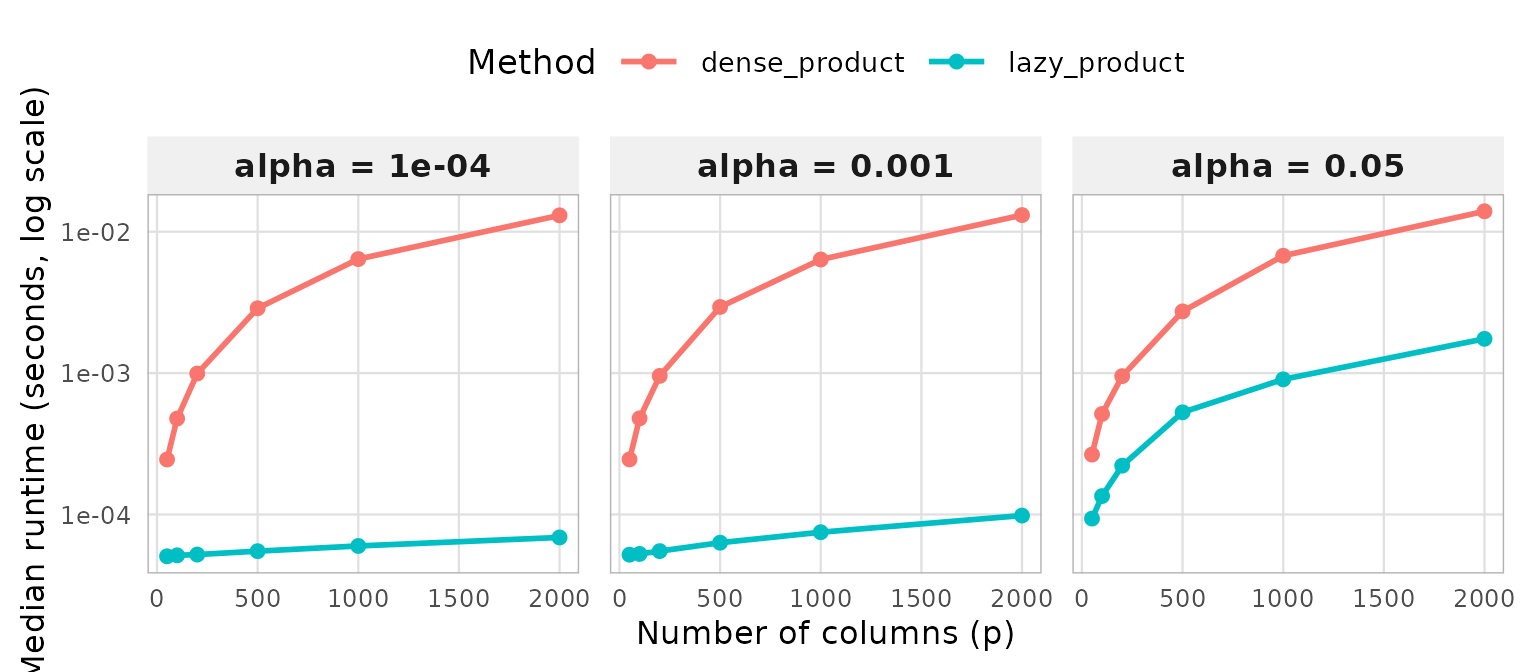

Each facet corresponds to a sparsity level, with the logarithm of median runtime on the vertical axis and the number of features $p$ on the horizontal axis. The red line represents the dense computation while the blue is the lazy computation. Looking at the figure, we note that dense computation requires $O(np)$ operations for the centering step, regardless of sparsity, since every element must be explicitly centered. This is confirmed in the plot, where the dense curve is identical across all three facets, increasing only with $p$ . The blue line representing the lazy computation however, shows clearly that computation time decreases as $\alpha$ gets lower. For $\alpha=0.05$ , the trend is similar to that of the dense computation, in the sense that as dimensionality gets higher, so does computation time. This follows from the $O(k + p)$ complexity of lazy computation, which approaches $O(np)$ as $\alpha$ increases. Conversely, as sparsity decreases and $k \ll np$ , the computational advantage of lazy evaluation becomes clear. Lazy computation exploits sparsity by operating only over the $k$ non-zero entries, avoiding the redundant computation on zero-valued elements that dense methods perform. Hence, the lazy computation gets better the sparser the matrix is, and also better the higher the dimensionality compared to dense methods.

Results of Memory Benchmark

The benchmark experiment is similar to that of computation time. We let $n$ be constant, augment $p$ and test for three levels of sparsity. Here, the measurements we make is the amount of memory used for storing the different objects.

#--------------------------------------------------
# Parameters
#--------------------------------------------------
n              <- 10000
sparsity_cols  <- c(0.05, 0.001, 0.0001)
p_values       <- c(50, 100, 200, 500, 1000, 2000, 5000)

#--------------------------------------------------
# Process results
#--------------------------------------------------
results <- list()
counter <- 1

for (sc in sparsity_cols) {
  cat("Running sparsity_col =", sc, "\n")
  for (p in p_values) {
    cat("  p =", p, "\n")

    M       <- create_sparsematrix_col(n = n, p = p, sparsity_col = sc)
    mem_res <- benchmark_memory(M)
    mem_res <- mem_res %>%
      mutate(sparsity_col = sc, n = n, p = p)

    results[[counter]] <- mem_res
    counter <- counter + 1
    rm(M); gc()
  }
}
#> Running sparsity_col = 0.05 
#>   p = 50 
#>   p = 100 
#>   p = 200 
#>   p = 500 
#>   p = 1000 
#>   p = 2000 
#>   p = 5000 
#> Running sparsity_col = 0.001 
#>   p = 50 
#>   p = 100 
#>   p = 200 
#>   p = 500 
#>   p = 1000 
#>   p = 2000 
#>   p = 5000 
#> Running sparsity_col = 1e-04 
#>   p = 50 
#>   p = 100 
#>   p = 200 
#>   p = 500 
#>   p = 1000 
#>   p = 2000 
#>   p = 5000

memory_results_col <- bind_rows(results) %>%
  mutate(mem_GB = mem_MB / 1024)

The results are presented in the following plot.

#--------------------------------------------------
# Plot for Memory Allocation
#--------------------------------------------------
ggplot(
  memory_results_col %>%
    mutate(sc_label = factor(
      paste0("alpha = ", sparsity_col),
      levels = paste0("alpha = ", sort(unique(sparsity_col)))
    )),
  aes(x = p, y = mem_GB, color = method, group = method)
) +
  geom_line(linewidth = 1) +
  geom_point(size = 2) +
  scale_y_log10(
    labels = scales::label_number(suffix = " GB", accuracy = 0.0001)
  ) +
  facet_wrap(~ sc_label, nrow = 1) +
  labs(
    x        = "Number of columns (p)",
    y        = "Allocated memory (GB, log scale)",
    color    = "Method"
  ) +
  vignette_theme(13)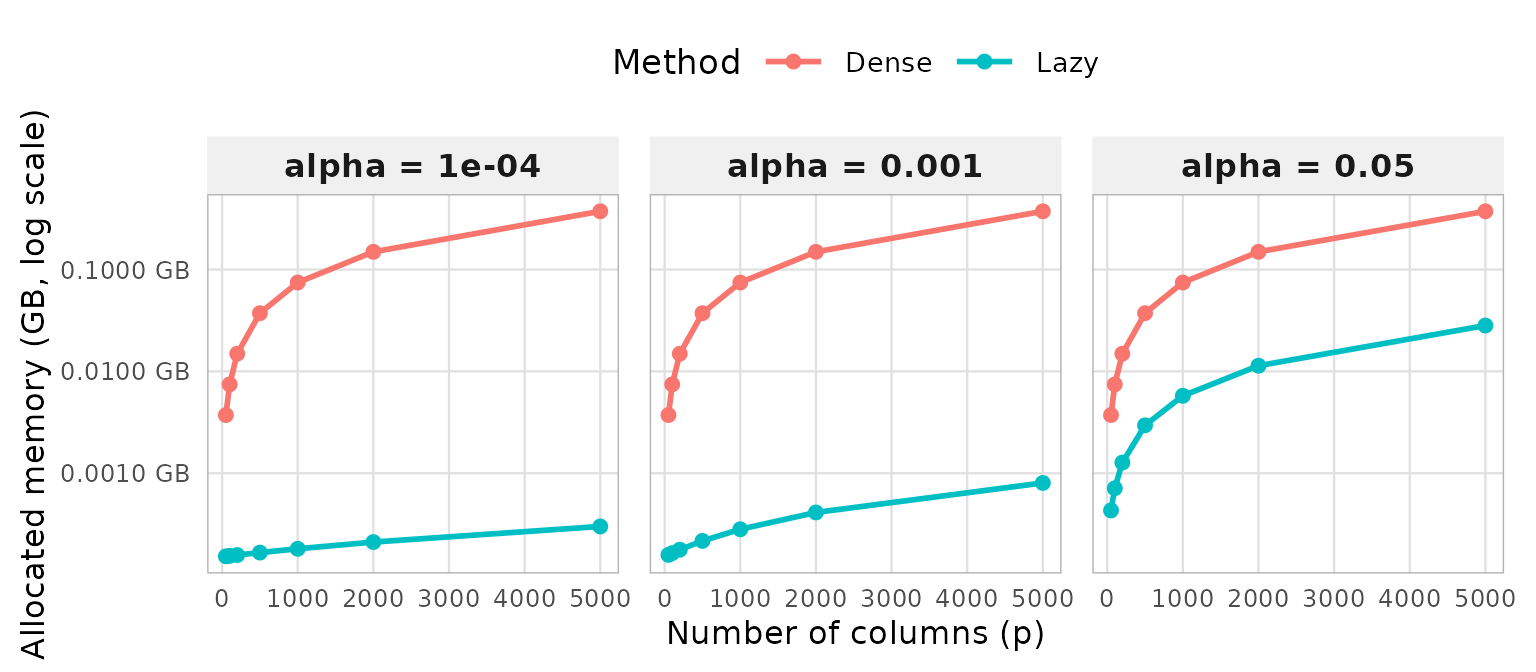

Each facet corresponds to a sparsity level, with the logarithm of median runtime on the vertical axis and the number of features $p$ on the horizontal axis. The red line represents the dense memory consumption while the blue is the lazy object’s. A key motivation for lazymatrix is the memory inefficiency of explicitly materializing normalized matrices. We therefore construct a memory benchmark under the same experimental setting as above, measuring memory usage rather than computation time. The dense representation requires $O(np)$ memory regardless of sparsity, as centering destroys the sparse structure and forces a full materialization of the matrix. As expected, the dense representation grows linearly in memory with increasing dimensionality. The implication being that using dense methods is infeasible for larger-scale data. The lazy representation follows a similar growth pattern at $\alpha = 0.05$ , as the data matrix and its associated location and scale parameters together require $O(k + p)$ memory, and $k$ remains large relative to $np$ at high sparsity levels. As sparsity increases, however, $k \ll np$ and the lazy representation retains significantly fewer bytes, directly reflecting the theoretical memory complexity established earlier. For the sparsest facet, memory consumption still grows with $p$ but remains orders of magnitude smaller than the dense representation across all three dimensions. In applications, high dimensionality and high sparsity tend to be correlated, hence it is crucial for LazyMatrixto perform well with the two parameters considered.

Performance of lazymatrix

Helper Functions

Results of Computation Time Benchmark

Results of Memory Benchmark

Performance of `lazymatrix`